If you have spent your career maintaining ATSC 1.0 transmitters, you know the drill: tune to the 8-VSB carrier, check forward power, glance at SNR and MER, and make sure the shoulders stay tucked under the emission mask. If those numbers line up, you are almost always good to go.
ATSC 3.0 (NextGen TV) completely changes the game.
With COFDM modulation, multiple Physical Layer Pipes (PLPs) carrying completely different constellations within the same 6 MHz channel, and forward error correction that masks degradation until the picture abruptly drops off a cliff, legacy test methods simply cannot keep up. When you are looking for an RF analyzer for ATSC 3.0, you need an instrument that goes well beyond surface-level carrier power. You need visibility into the physical layer parameters that actually tell you how your transmitter, antenna system, and coverage area are behaving, so you can fix problems before viewers notice a glitch.
Whether you are commissioning a new exciter, balancing a Single Frequency Network (SFN), or setting up 24/7 remote site monitoring, here is what truly matters when evaluating an RF analyzer ATSC 3.0 engineers can depend on, illustrated with real measurement screens along the way.
Screenshots throughout show representative WebGUI views from ATSC 3.0 signals captured across different test configurations.
1. Core RF Measurements: What an ATSC 3.0 RF Analyzer Must Deliver
Everything starts with the RF signal itself, but the multi-carrier nature of ATSC 3.0 demands far more precision and dynamic range from your test receiver than older single-carrier gear ever required.
Calibrated Absolute Power (dBm) and Modulation Error Ratio
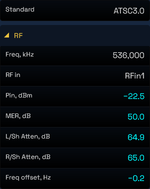
A dependable RF analyzer for ATSC 3.0 has to provide calibrated, absolute signal levels in dBm (or dBµV) across the occupied channel bandwidth, not an arbitrary percentage bar. Whether you are sampling a 50 dB directional coupler at the transmitter output or measuring an off-air antenna during a field survey, you need real numbers to verify high-power amplifier (HPA) gain and track path loss accurately. Paired with that, a Modulation Error Ratio (MER) measurement gives you your first reliable baseline of raw channel quality.
Practical Engineering Note: Match Your Input Level to the Calibration Point
Every receiver front-end has an optimal operating window. If the RF input into the analyzer is driven too hard, you risk pushing the front-end into non-linear distortion, generating false intermodulation products and artificially degrading your measured MER and spectrum shoulders. In other words, the analyzer starts measuring its own distortion instead of your transmitter's. If the signal is padded down too low, you push the measurement closer to the instrument's thermal noise floor.
The fix is simple: find out what input level your analyzer was calibrated at, and adjust your directional coupler pads and inline attenuation to deliver that level at the RF input port.
Under FCC 47 CFR §73.1590 (and equivalent international broadcast rules), stations are legally obligated to keep emission records and maintain strict compliance with transmission masks. As high-power amplifiers warm up, age, or operate near saturation, non-linearities create intermodulation distortion that shows up as spectral regrowth ("shoulders") at the channel edges.
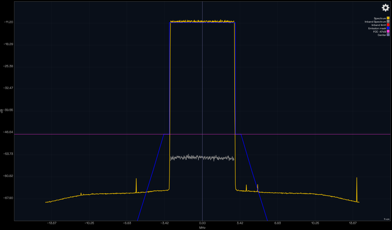
An ATSC 3.0 RF analyzer needs to calculate upper and lower shoulder attenuation automatically against standard regulatory masks. Generating timestamped, exportable logs of these shoulders protects your station during compliance reviews and lets you verify that your exciter's digital adaptive pre-correction (DAPC) is doing its job.
The blue trace is the emission mask. What matters is the gap between the signal's shoulders and the mask edge - that margin disappears first as an amplifier ages or drifts toward saturation.
Practical Engineering Note: Don't Assume the Default Mask Is Your Mask
Analyzers typically ship configured to the standard FCC-defined emission mask. But regulatory emission limits vary across international jurisdictions and frequency band allocations. If you operate outside the U.S., or under specific license conditions, verify that the mask your analyzer is testing against actually matches your national standard or license parameters.
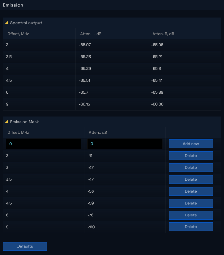
A mask is defined by a series of breakpoints, each pairing a frequency offset with the attenuation required at that offset. Being able to edit those individual breakpoints is what lets you model any jurisdiction's limits accurately, as shown below.
A mask is nothing more than this list: offset in MHz, required attenuation in dB. The upper table shows measured spectral output at the same offsets, so you can compare measurement against limit point by point.
Carrier Frequency Offset and Sample Rate Shift
In ATSC 3.0, subcarriers in 16K or 32K FFT modes are packed tightly together. A slight local oscillator (LO) drift in your exciter can cause inter-carrier interference (ICI) that degrades MER across the entire multiplex. Your analyzer should continuously track:
Carrier Frequency Offset (Hz): Catches exciter reference drift early.
Sample Rate Shift (Hz): Flags timing mismatches in D/A and A/D conversion stages before demodulation fails.
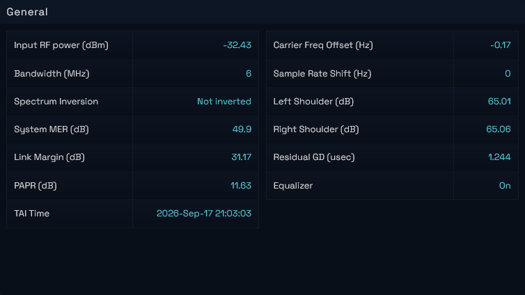
-0.17 Hz offset and zero sample rate shift is a well-disciplined exciter. Watch these as a trend rather than a snapshot - the trend is what tells you a reference is drifting.
Practical Engineering Note: Measure Against the Same Clock Your Transmitter Uses
For standalone applications or field surveys where a master site clock is unavailable, the analyzer depends on its internal timebase, which is why a high-stability Oven-Controlled Crystal Oscillator (OCXO) matters.
For 24/7 transmitter plant installations, supply an external 10 MHz reference, ideally the very same GPS/GNSS reference distributed to the monitored TV transmitter. The reason is simple: if the analyzer and the exciter share one reference, any frequency offset you measure is real exciter drift, not a disagreement between two independent clocks.
Always confirm which reference is actually active. If an external reference drops out and the analyzer falls back to its internal oscillator, the meaning of your frequency measurements changes. The System Information page below shows the active reference source at a glance.
Running on the internal OCXO - correct for a field survey, and also what you'd see if an external reference dropped out at a transmitter plant.
2. Demodulation Depth: Why an RF Analyzer for ATSC 3.0 Needs Per-PLP MER
In ATSC 1.0, you had a single MER reading for the whole channel. If it read 28 dB or better, you could sleep soundly. Try that in ATSC 3.0, and you could be facing an outage without warning.
The Pitfall of Average Channel MER
ATSC 3.0 multiplexes multiple Physical Layer Pipes (PLPs) into a single RF channel. Each pipe can be configured with its own modulation order, code rate, and time-interleaving depth:
A rugged pipe might run QPSK or 16QAM aimed at mobile receivers or emergency alerts.
A high-capacity pipe might push a dense 256QAM or 1024QAM constellation delivering high-throughput 4K UHD.
These two pipes have completely different reception thresholds. The QPSK pipe might decode cleanly at 12 dB MER, whereas the 256QAM pipe could fail below 24 dB.
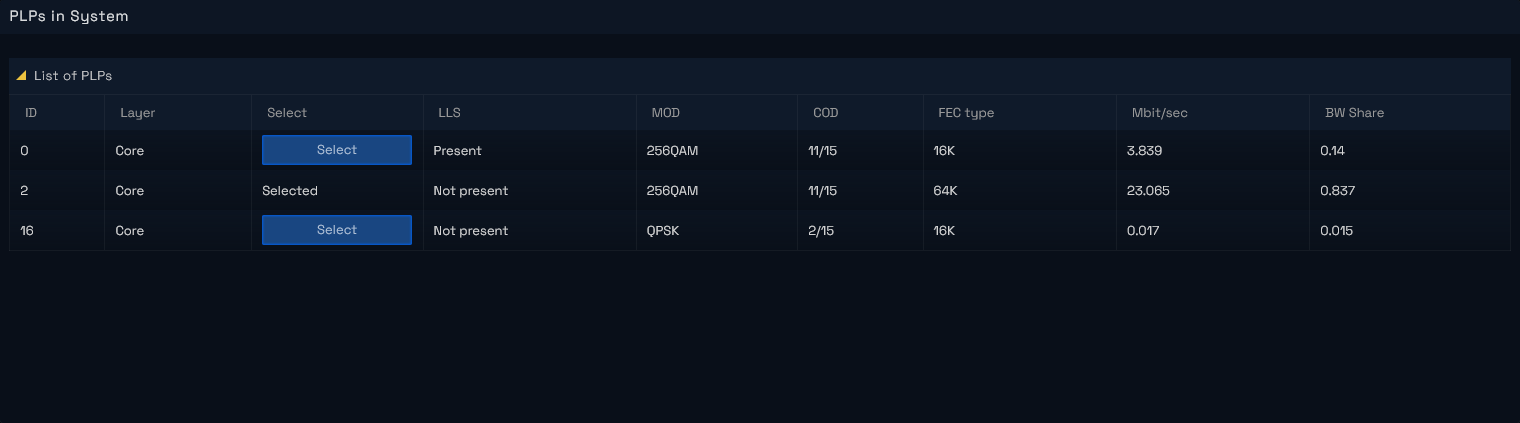
Three pipes in one 6 MHz channel. The 256QAM pipe carries 23 Mbps across 84% of the bandwidth; the QPSK 2/15 pipe carries 0.017 Mbps and is built for ruggedness. They will not fail at the same signal level.
If your analyzer only reports an average MER across the whole channel (say, 26 dB), it looks acceptable on the surface. But that number could easily hide the fact that your high-capacity PLP is sitting right on the verge of total failure. An effective RF analyzer ATSC 3.0 must peel back the layers and report separate MER for:
Bootstrap Preamble
L1-Basic Signaling
L1-Detail Signaling
Each Active PLP independently
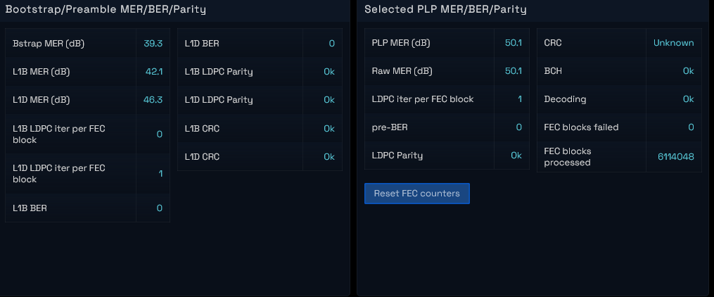
MER is reported per selected pipe, alongside independent bootstrap and L1 readings. Select a different PLP and this panel reports that pipe instead - on a degraded signal they can differ by several dB.
Multi-Layer Constellation Diagnostics
When MER drops, the fastest way to understand why is the I/Q constellation diagram. Constellation patterns point straight to the root cause: circular blurring points to local oscillator phase noise, an oval stretch indicates I/Q gain or quadrature imbalance, and squashed outer corners on a 256QAM plot reveal amplifier compression.
Because ATSC 3.0 uses different modulations across signaling blocks and data pipes, a capable analyzer must provide discrete constellation views for every layer of the transmission.
Practical Engineering Note: Which Constellations to Check, and What Each Tells You
In ATSC 3.0, modulation analysis means inspecting service-level pipes and physical-layer signaling independently. A practical workflow is to list all active PLPs in the multiplex, select the pipe you are concerned about, and review its statistics (modulation scheme, code rate, time interleaving, and dedicated MER) alongside its constellation. From there, five constellation views cover the full signal:
Selected PLP Constellation: The chosen pipe's I/Q symbol grid (from QPSK up to 4096QAM). This is where service-level impairments show up first.
Core + Enhanced Constellation: Visualizes layered symbol structures when operating with Layered Division Multiplexing (LDM).
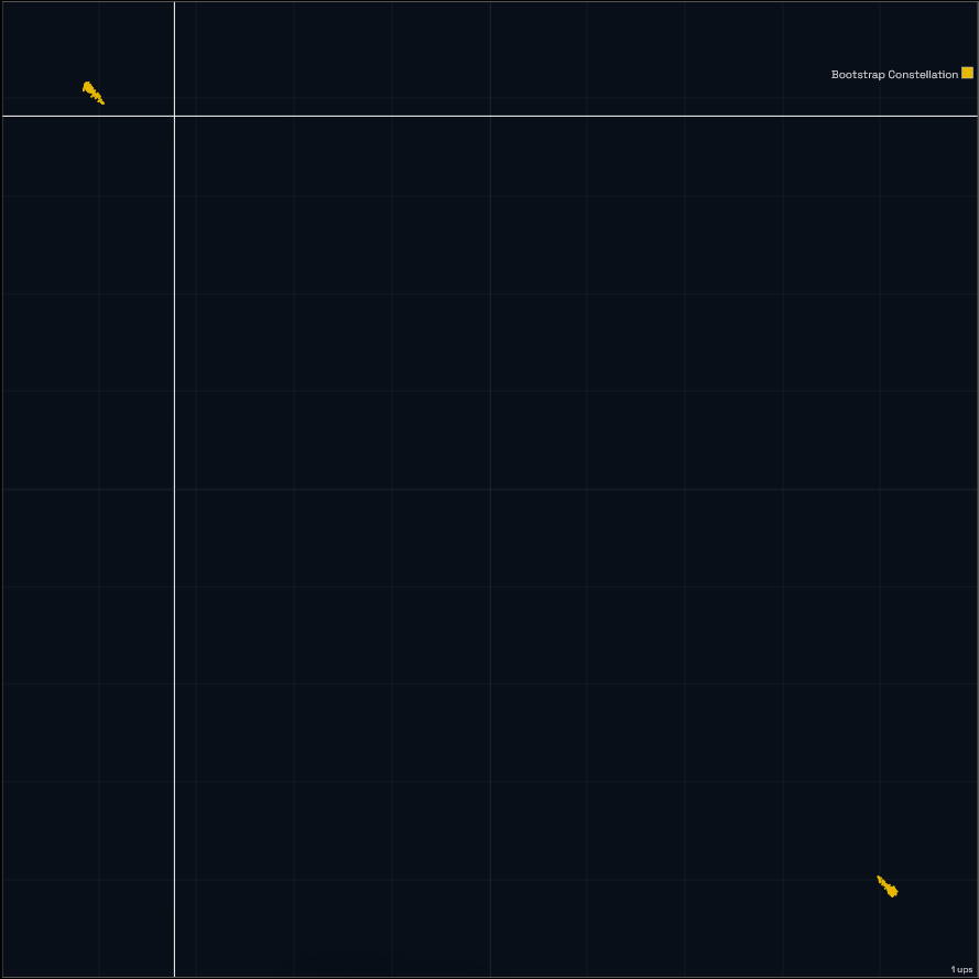
Bootstrap Constellation: Verifies the modulation accuracy and synchronization stability of the initial system preamble.
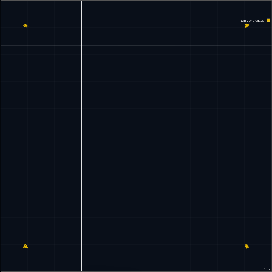
L1B Constellation: The symbol constellation of the L1-Basic signaling block.
L1D Constellation: Modulation integrity for the L1-Detail signaling layer.
Three of those views are shown below. The Selected PLP and L1-Detail views work identically - same plot, different layer of the signal.
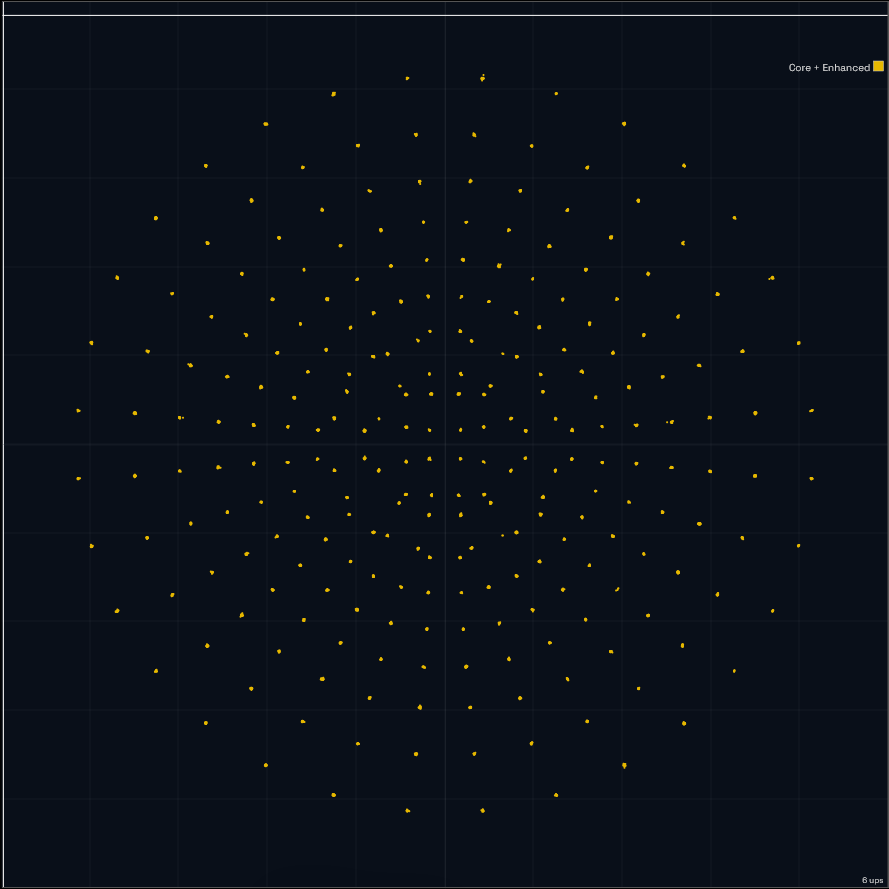
A layered (LDM) constellation. Points are tight and evenly separated - impairments show up as blurring, stretching, or compression of the outer points.
The bootstrap preamble uses an extremely rugged modulation, which is why it survives down to -6 dB SNR. Very few symbol states, spaced as far apart as possible.
Four tight clusters. If these start to smear while your data pipe still looks clean, the problem is in the signaling layer, not the service.
3. Forward Error Correction: LDPC Iteration Tracking in an ATSC 3.0 RF Analyzer
Digital signals don't degrade with visible "snow." They look pristine right until they freeze. This "cliff effect" makes traditional Bit Error Rate (BER) monitoring insufficient on its own.
The Limit of Post-LDPC BER
ATSC 3.0 uses Low-Density Parity-Check (LDPC) error correction paired with an outer BCH code. The LDPC decoder works iteratively, crunching parity equations over multiple cycles to resolve corrupted bits.
If you only monitor Post-LDPC BER, it will read zero when your link budget has 15 dB of headroom, and it will still read zero when you have only 0.5 dB of margin left. You know the signal is currently decoding, but you have no idea how close you are to the edge of the cliff.
LDPC Iterations: Your Real-Time Early Warning System
Tracking the number of LDPC decoder iterations solves this problem. The average number of iterations over time is a continuous function of signal SNR, which is exactly what post-LDPC BER is not - it sits at zero until it doesn't. Exact figures depend on the decoder's maximum iteration setting, but the pattern is consistent:
Low, stable iterations: The decoder resolves codewords effortlessly. Your link budget is healthy.
Climbing iterations: Noise, multipath, feeder cable water ingress, or amplifier drift is forcing the decoder to work significantly harder.
Nearing the ceiling: When iterations approach the decoder's maximum limit, uncorrectable errors and macroblocking are about to strike.
The per-PLP panel shown earlier reports iterations per FEC block alongside pre-BER and a running count of failed blocks. A single iteration per block across millions of processed blocks with zero failures is a signal with comfortable headroom. Avateq's ATSC 3.0 RF signal analyzer performance test examines this relationship in detail against the theoretical limits in A/327.
By watching iteration trends over time in your RF analyzer ATSC 3.0 dashboard, you spot degrading RF conditions hours or days before an on-air failure, letting you plan a routine site visit instead of responding to an emergency truck roll at 2 a.m.
Capacity vs. Robustness: Reading a Link Margin Analysis
Monitoring degradation protects you against unexpected outages, but ATSC 3.0 also gives broadcasters an opportunity to optimize transmission capacity. Station engineers constantly balance robustness against throughput: can we afford to upgrade a PLP's modulation to launch an additional HD stream or high-value datacasting service without compromising reception reliability?
Normally, answering that question involves digging through technical standards, manual math, and guesswork.
Practical Engineering Note: Evaluate Upgrades Against the Live Signal
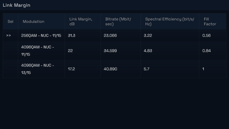
A faster approach is a link margin analysis: take the live incoming RF signal and calculate how much reception margin each candidate modulation and code rate would leave under current conditions. The result is a side-by-side table of five metrics:
Modulation & Code Rate: The active scheme (marked with >>) compared against higher-capacity alternatives.
Link Margin (dB): Remaining reception margin under current live RF conditions for each configuration.
Bitrate (Mbit/sec): Projected net data throughput for each option.
Spectral Efficiency (bit/s/Hz): Bandwidth efficiency across the channel.
Fill Factor: Channel utilization, from baseline up to 1.0 (100%).
256QAM 11/15 at 31.3 dB margin and 23.07 Mbps; 4096QAM 11/15 at 22.0 dB and 34.60 Mbps; 4096QAM 13/15 at 17.2 dB and 40.89 Mbps. Stepping up adds 50% throughput and costs 9.3 dB of margin.
Reading the table above: stepping up from 256QAM to 4096QAM (11/15) increases throughput by 50%, from 23.07 Mbps to 34.60 Mbps. That costs 9.3 dB of margin, but still leaves a robust 22 dB. Pushing further to 13/15 fills the channel completely (fill factor 1.00) and leaves 17.2 dB. Whether that last step is worth it depends on how much margin your coverage area actually needs for fading, indoor reception, and mobile viewers.
4. Bootstrap and L1 Signaling Protocol Decode
Before an ATSC 3.0 receiver can demodulate program content, it has to acquire and parse the signal's underlying signaling structures.
Bootstrap Structural Validation
The ATSC 3.0 Bootstrap (ATSC A/321) is an ultra-rugged preamble designed to be picked up even below the noise floor (down to -6 dB SNR). It handles initial synchronization and carries emergency alert wake-up bits. An ATSC 3.0 RF analyzer must validate that the bootstrap waveform is structurally sound, timing-accurate, and compliant with standard versioning.
L1-Basic and L1-Detail Parsing
Following the bootstrap, the physical layer frames convey two critical signaling stages:
L1-Detail: Specifies the complete technical configuration for every subframe and PLP, including modulation, code rates, time interleaving, and antenna modes.
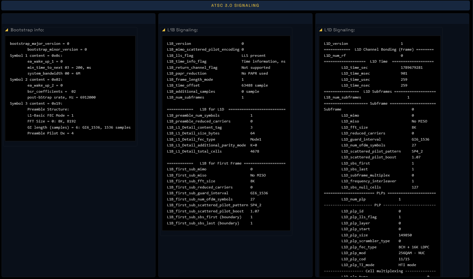
An analyzer should decode and display these tables clearly. When you update exciter firmware or adjust your broadcast gateway scheduler, checking the live decoded L1 table ensures that the signal radiated over the air matches your engineering plan, preventing subtle receiver incompatibilities in the field.
Every parameter your scheduler configured, read back off the air: FFT size, guard interval, scattered pilot pattern, per-PLP modulation and code rate. Check this page after a firmware or gateway change.
5. OFDM Pilot Analysis, Channel Impulse Response, and SFN Timing
Single Frequency Networks (SFNs) allow broadcasters to cover complex terrain and improve building penetration by broadcasting on the same RF frequency from multiple towers. But tuning an SFN requires careful control over arrival times.
Scattered Pilots and Channel Estimation
ATSC 3.0 embeds reference pilot carriers throughout the OFDM grid based on 16 standardized scattered pilot patterns (SP3_2 through SP32_4). A dedicated ATSC 3.0 RF analyzer tracks these pilots to compute channel estimation across the band.
Channel Impulse Response (CIR) and Echo Profiling
Applying an inverse FFT to those channel estimates yields the Channel Impulse Response (CIR), essentially a time-domain profile of all incoming signal arrivals:
Main Path: The primary signal arrival.
Pre-Echoes: Arrivals landing before the main path (often from closer repeaters or nearby reflections).
Post-Echoes: Delayed arrivals bouncing off hills and buildings, or coming from distant SFN nodes.
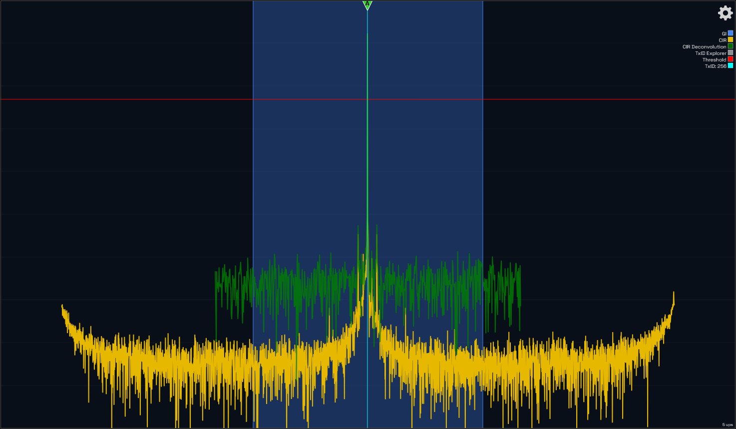
Reference case: single-transmitter reception with no significant multipath. One arrival inside the guard interval, nothing above the threshold line.
Keeping Echoes Inside the Guard Interval
In a properly synchronized SFN, secondary transmitter arrivals must land inside the OFDM symbol's Guard Interval (GI). When they do, they combine constructively and boost signal strength. If an echo slips outside the GI, it turns into destructive co-channel interference and tanks your MER.
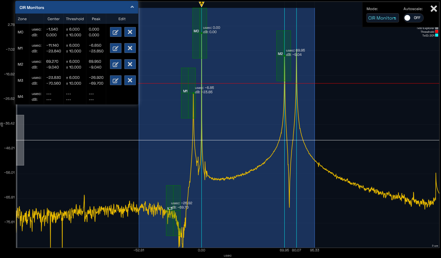
Three arrivals: main path at 0 µs, a pre-echo 6.85 µs early at -23.85 dB, and a second transmitter 69.95 µs late at only -9.04 dB. All inside the guard interval - but that late arrival has ~10 µs of margin before it turns destructive.
A CIR display lets you:
Measure the exact delay (µs) and relative amplitude (dB) of every transmitter arrival.
Confirm that network delay offsets set at your broadcast gateway match real-world arrival times.
Catch GPS/GNSS timing reference drift at remote transmitter sites before synchronization slips outside the guard interval.
6. Continuous 24/7 Monitoring and Telemetry Integration
Portable test sets are great for field surveys, but transmitters rarely give you advance notice before failing. Gradual degradation (a cooling fan failing, an amplifier module drifting out of bias, or water slowly seeping into a coaxial connector) demands continuous, automated oversight.
What an Always-On Monitoring Receiver Must Do
When installing an RF analyzer for ATSC 3.0 permanently at the transmitter plant, look for:
Rugged Rackmount Hardware: Designed for continuous operation in high-RF environments.
Automated Logging for FCC Compliance: Persistent recording of signal levels, shoulders, and MER to meet 47 CFR §73.1590 requirements without manual intervention.
Modern Telemetry Protocols: Built-in support for SNMP v2c/v3, MQTT (JSON formatting), and REST APIs so data feeds directly into your station's Network Operations Center (NOC).
Correlated Event History: When an alarm trips at 3 a.m., a simple "MER Low" message doesn't tell you the story. You need to see what the signal parameters looked like immediately before, during, and after the alarm, ideally alongside any maintenance activity logged on the same timeline.
ATSC 3.0 RF Analyzer Evaluation Checklist
Use this practical checklist when reviewing any RF analyzer ATSC 3.0 monitoring receiver or test instrument for your facility:
Measurement Domain
Key Required Feature
Why It Matters Operationally
RF Physical Layer
Calibrated absolute level (dBm), system MER
Accurate forward power verification and survey path-loss calculation
Direct integration into station NOC dashboards without proprietary software
Compliance History
Persistent internal logging with correlated alarm capture
Full before/after signal context when diagnosing incident causes
Conclusion: Choosing the Right RF Analyzer for ATSC 3.0
ATSC 3.0 is a remarkably capable broadcast standard, but its layered physical architecture means surface-level measurements are no longer enough. To run a stable, compliant, and optimized transmission plant, broadcast engineers need an analyzer that looks into every layer of the signal stack: from the bootstrap and L1 signaling, through per-PLP modulation quality, to LDPC decoder iterations and SFN echo profiles.
Selecting an RF analyzer for ATSC 3.0 engineered around these physical-layer realities gives your team the visibility to catch equipment drift early, commission SFNs with confidence, and maintain rock-solid reliability across every service you broadcast.
How Avateq Approaches ATSC 3.0 RF Analysis
Every screenshot in this guide was captured on Avateq instruments, which were designed around the measurements covered above.
AVQ1020 - RF Layer Monitoring Receiver: Built for uninterrupted 24/7 transmitter plant operation, with continuous calibrated power, MER, automated shoulder attenuation calculations, and real-time frequency and clock drift tracking.
AVQ1022 - RF Signal Analyzer: Everything in the AVQ1020, plus the complete multi-layer constellation suite with granular per-PLP statistics, and built-in OFDM pilot analysis with real-time echo profiling for commissioning and maintaining SFN installations. Also available as the AVQ1022M, a mobile version with two RF inputs for field work.
AVQ200 - RF Signal Inspector: A compact unit carrying the same multi-layer constellation suite and per-PLP statistics, built for in-field analysis and SFN/off-air monitoring.
Across the lineup, Avateq units share the details that make these measurements dependable:
FCC emission mask by default, with editable breakpoints in the user interface for any jurisdiction or license.
Internal OCXO with automatic external 10 MHz sensing: connect an external reference and the unit locks to it automatically, with the active source shown on the System Information page of the WebGUI.
LDPC iteration tracking and code-block BER, alongside the Link Margin Analysis engine in the WebGUI
Metrics Logging Engine: runs on the receiver, logs all physical-layer metrics, streams updates to visualization tools like Grafana over HTTP, records alarms with the surrounding signal data, and provides an API for logging maintenance notes directly into the timeline.
Setup procedures, firmware notes, and measurement definitions for every unit are documented in the Avateq online manual.